OpenMetrics & Prometheus Primer

One thing i’ve been heavily exposed to across a lot of organizations is general observability strategy

I’ve worked with various SaaS offerings including DataDog, AppDynamics, and the various native cloud offerings and hybrid packaged models like Elastic, alongside various native cloud provider logging solutions like AWS CloudWatch and GCP StackDriver.

I’m a big advocate of Open Source Software and have generally been a proponent of the OpenMetrics standard, and the general approach to lower cost monitoring by pre-computing time-series data structures as opposed to indefinite storage of traditional log-based solutions with heavy indexing.

Ultimately this has led to a few different open source contributions across projects largely in the web3 space, namely the Ethereum Prysm Client to participate in the execution layer of the network, and the MEV-Boost project a tool used by node operators to coordinate block preparation to extract rewards via relays.

We’ll talk a little about those contributions an how you might end up getting involved in OSS like this in future, as well as a suggestion for some low hanging fruit in those repositories, but first in this post we’ll start delving into the underlying wire format for OpenMetrics, and the implications of using this as a primary datasource for Prometheus.

Caveats

The aim of this is to not go too far into the underlying implementation, but more so into the standard and how it is used practically from an engineering perspective.

This post will touch on the high level OpenMetrics spec, if you’re familiar with prometheus, there’s probably not a huge amount of new info here, it’s intended to get folks up to speed ahead of some more deep-dive content.

What is the OpenMetrics Standard?

A metric represents a single point from a time series, put simply; a single point from a line on a line graph. The OpenMetrics standard looks to standardize this by going a step further and suggesting the wire format, the collection standards and the exposure of these metrics. Following this standard will plot you a line on a graph.

The format is flexible enough to support various types of data types, which at a super high level are as follows:

Counter

Represents an increasing counter, the value can only ever go up, use this to represent things like # of times an event has occurred, this is probably the most used metric type and the really standard example for this is an API request counter.

api_request_count{path="/health"} 10

Breaking this down further, the above metric tells us that we have made 10 requests to the /health endpoint of our service.

Gauge

Can go up and down, used commonly to represent percentages or a live value, for example % disk usage, usually suffixed with _meter

disk_used_percent{mount="/",disk="rootfs"} 0.127

This metric tells us the current percent disk usage as a decimal for the specified mount and disk at 12.7%

Histogram

A complex metric type, a histogram creates multiple metrics, it’s used to separate time-series into buckets, you’d use this to represent durations i.e. request latency

api_request_latency{path="/health",le="0} 0
api_request_latency{path="/health",le="10} 10
api_request_latency{path="/health",le="100} 12
api_request_latency{path="/health",le="1000} 5
api_request_latency{path="/health",le="2000} 1
api_request_latency_sum{path="/health",} 8524
api_request_latency_count{path="/health"} 28

Let’s take the metrics that have an le label, what we’re doing is increasing the counter for each labelled bucket for each request latency that falls into that bucket, so from this, we can see that le=1000 having a value of 5 means that we’ve seen that latency 5 times overall.

Usually, this is implemented through an abstraction in the implementing SDK, in GO it’s using the .Observe() method, this will automatically bucket things into the pre-defined buckets

Histograms have had the most notable changes in terms of architecture, but i won’t go into detail about that in this post.

Logs to Metrics

One tool i’ve found great to ease the transition into prometheus metric production is using “grok-exporter”, the principle is to parse structured logs and count occurrences of patterns, for example from the following logs

{time="1658934286", method="get", endpoint="/api/v1/nodes"}
{time="1658934287", method="delete", endpoint="/api/v1/nodes"}
{time="1658934288", method="get", endpoint="/api/v1/nodes"}
{time="1658934290", method="get", endpoint="/api/v1/nodes"}
{time="1658934290", method="get", endpoint="/api/v1/nodes"}
... +96 more

We could look to produce the following metrics

http_requests_total{method="delete",endpoint="/api/v1/nodes"} 1
http_requests_total{method="get",endpoint="/api/v1/nodes"} 100

One of many shameless plugs in this series, here’s a repository I put together a while back (0xste/grok-exporter) to containerize another project. (fstab/grok-exporter)

You can make use of the configuration below to parse a simple json formatted log, or alternatively a more comprehensive example including separating out the parser configuration is found in this proposed contribution to MEV-Boost. This came around because implementing full prometheus instrumentation is a very deep change to the codebase, and is run on 1,000s of validators, so in an aim to circumvent the latency involved in getting a large change onto the main branch, this works as a stopgap.

The below points to a log file and exports a counter metric by counting the log lines that match the corresponding “grok” pattern, of which we can also reference some pre-defined patterns. We can reach this prometheus server on port 9144.

global:
  config_version: 3
input:
  type: file
  paths:
    - ./my-log-file.log
  readall: true
  fail_on_missing_logfile: true
imports:
  - type: grok_patterns
    dir: ./patterns
metrics:
  - type: counter
    name: http_requests_total
    help: The the number of http requests
    match: 'endpoint=%{URIPATH:path}'
    labels:
      path: '{.endpoint}'
server:
  port: 9144

Check yourself before you wreck yourself

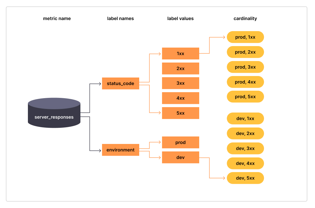
Cardinality

One of the main care points is that every unique combination of key-value label pairs represents a new active time series, which can dramatically impact performance over a number of dimensions, namely: storage, query performance and collection delay.

Cardinality is a measure of how many distinct occurances of the “fingerprint” of you rmetric. So for example a label containing HTTP methods would have a cardinality of 2 if you had only GET and POST in your application, which is usually fine given there’s a finite set of available HTTP methods. A http path is a good example of bad metric cardinality in most instances, and is not something you’d generally use as a label, instead, you’d favor something like an OpenAPI OperationID to identify the route as opposed to the full path, again, reducing the set of possible values.

It’s generally advised not to use labels with high cardinality (many different label values), such as user IDs, email addresses, or other unbounded sets of values.

This can grow to be incredibly unwieldly from an operations POV, and is always something that engineers should keep in mind when using the various SDKs, as for the most part, there are no guard rails!

Prometheus & OpenMetrics

While we’ve not really mentioned Prometheus yet, we’ll dig into the practical aspects of running a local server so we can start to get familiar with things.

While it’s quite an obtuse term, Prometheus today covers a lot of use-cases, but primarily when i use the word, i’m referencing it’s usage as a storage system, however provides quite a few additional capabilities, including ingestion, discovery and alerting.

For the purposes of this blog, we’ll look primarily at the Database elements from a practical applied perspective as opposed to operational aspects.

Prometheus

Prometheus is many things, for the purposes of this section, i’m going to refer to it largely in the context of a time series database, however it supports a wide array of things outside of that scope, including but not limited to metric ingestion, service discovery, it’s own query language PromQL, a GUI for visualizing queries, and it’s on baked-in alerting system. All of which combine to provide a flexible ecosystem of tools that are simple to get started with.

In this section, we’ll take a practical look at the latest version of prometheus, and explore some of the new features.

Getting Started

To start using Prometheus, you typically:

1. Deploy the Prometheus server
2. Configure Prometheus to scrape metrics from your targets
3. (Optional) Set up Alertmanager for notifications
4. (Optional) Connect Grafana or another visualization tool for dashboarding

1. Deploy Prometheus

Going to assume you have docker running on your machine, if not the setup guide here should cover you.

We need to write some configuration for prometheus, but the default will do us for now, by default we’ll register the metamonitoring endpoint i.e. metrics from the underlying prometheus server.

We’ll make use of the latest version of prometheus that’s still in beta, it gives us a shinier UI as well as some OpenTelemetry features we’ll look at later in the series

# run prometheus server
docker run -d \
    -p 9090:9090 \
    -v prometheus-data:/prometheus \
    --network appnet \
    --name prometheus \
    prom/prometheus:v3.0.0-beta.0

This will start a prometheus server, expose the UI on localhost:9090, ensure that any metrics ingested are persisted to disk, create a docker overlay network called appnet and launch a container called prometheus

We can check this by running docker ps

We can open up localhost:9090 in a browser, and we can have a poke around the configuration ui

We can even begin to run some queries on the native prometheus metrics, but we can revisit this soon.

2. Configuring our app

Given we’re launching prometheus in docker, we’ll make use of docker networking, so for our app from the previous post, we’ll make use of the following dockerfile. For our purposes this will do for this purpose

# syntax=docker/dockerfile:1
FROM golang:1.23-alpine as BUILD
WORKDIR /src
COPY . .
RUN ls -ltra
RUN go build -o /bin/blog ./main.go

FROM alpine:3.20
COPY --from=BUILD /bin/blog /bin/blog
CMD ["/bin/blog"]

We can then build and deploy this locally following something like

# create the network, we'll use this later
docker network create --attachable -d bridge appnet

# build image
docker build -t 0xste/blog-api .

# run and expose app and prometheus ports in the appnet
docker run -d --network appnet -p 9000:9000 -p 8080:8080 --name blog-api 0xste/blog-api

2. Configuring a scraper

We can now look at applying a configuration to retrieve from the above published metrics endpoint.

We can create a file at ./config/prometheus.yml, the part to note is that because we’re using docker networking, we’re using the bridge network we defined above to communicate with blog-api container using the container name.

# my global config
global:
  scrape_interval: 10s
  evaluation_interval: 10s

scrape_configs:
  - job_name: prometheus
    static_configs:
      - targets:
          - localhost:9090
  - job_name: 0xste_blog
    static_configs:
      - targets:
          - blog-api:9000

We can then follow the same process as above, in which we run and start our prometheus endpoint, note the command below references the configuration explicitly and mounts it to the container.

# run prometheus server
docker run -d \
    -p 9090:9090 \
    -v ${PWD}/config/prometheus.yml:/etc/prometheus/prometheus.yml \
    -v prometheus-data:/prometheus \
    --network appnet \
    --name prometheus \
    prom/prometheus:v3.0.0-beta.0

If we jump back into the UI by navigating to localhost:9090/targets we can see if our configuration is correct

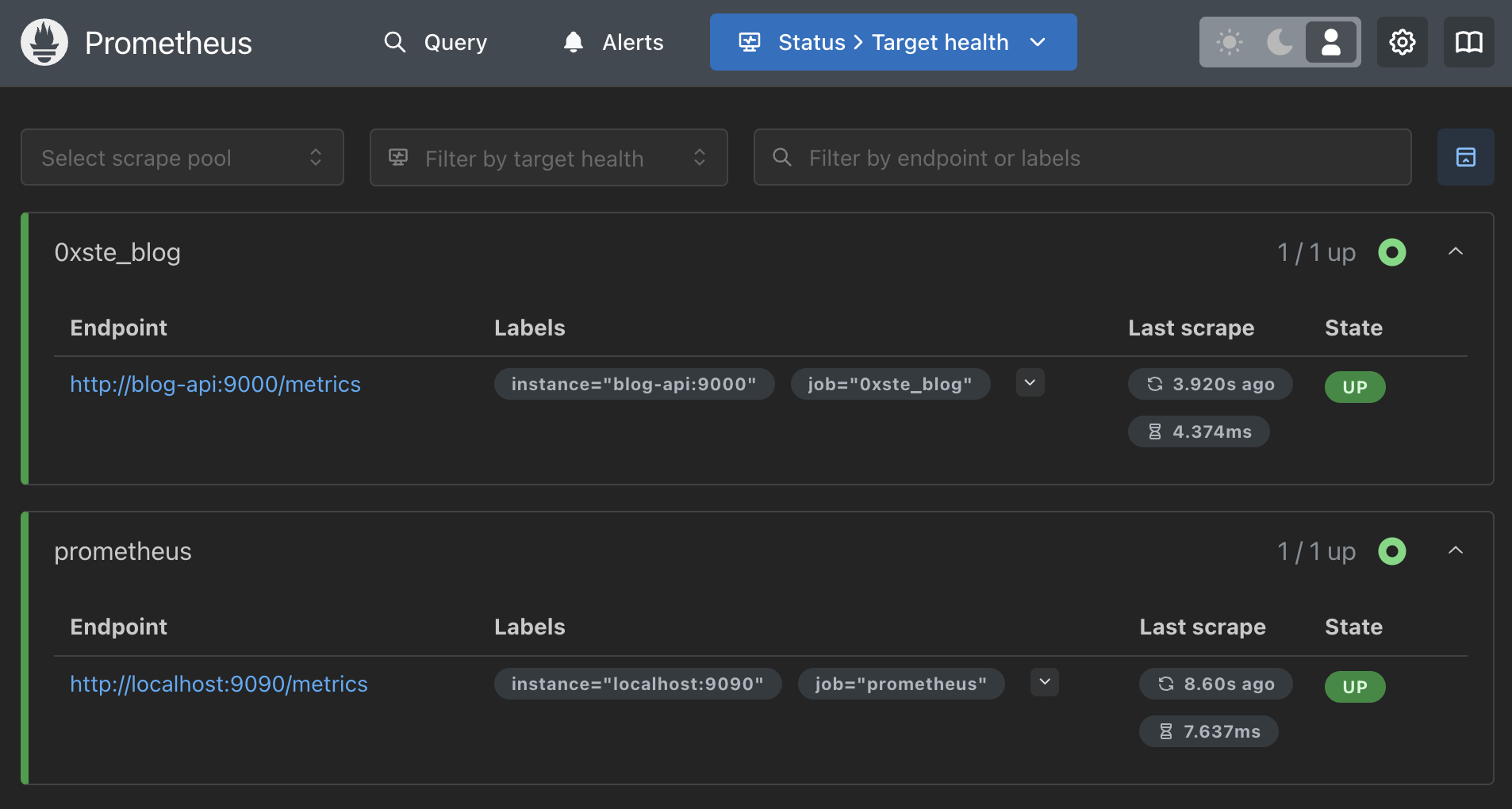
If we’re all green here, then we’re ingesting metrics!

PromQL

A lot of people diving deeper into these kinds of dashboards, or trying to implement themselves pretty quickly find themselves running into the main query language for Prometheus timeseries.

Anecdotally, engineers i’ve worked with on this agree that the learning curve for PromQL is… quite steep.

It may sometimes feel like you’re chained to a rock, having your liver pecked out by an eagle every day for eternity when trying to get a PromQL query to do what you expect it to. (a terrible mythology joke)

Query Basics

We’ll often see in UIs for metric query engines a few query options you can play around with

You usually see two types of queries:

• In grafana, it’s referred to as “Instant” or “Range”
• In Prometheus, it’s referred to as “Table” or “Graph”

we’ll usually see a overarching time filter in the top right of most query engines, to dictate the range of the query, which is different from the query range period, which we’ll get into a bit more later on in this guide.

Common Counter Queries

So let’s start with some basics, we’ll explore more nuance of the language later

So first, let’s make some requests to our api, opening a browser at localhost:8080/123 will suffice.

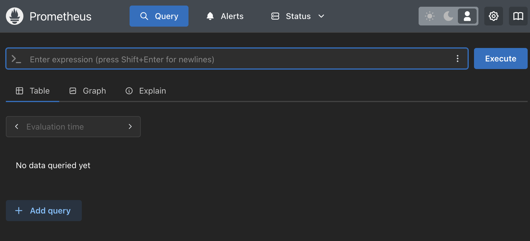
If we navigate to our query viewer in the GUI, we’ll be able to construct some queries

Requests by path over time

This function makes use of the increase operator, with a period of [30s], this tells the query engine to look only at the delta between the first and last value in a 30s contiguous period for a monotonically increasing counter.

The max by aggregation simply rolls up the labels across all metric series so we’re able to view only the labels we care about, this is not particularly relevant for our query, but may be as we scale up our queries

Simply, this will give us the overall count of requests by path

max by (path)(increase(http_request_count[30s]))

Overall API Uptime

If we wanted to take this a step further, we’d look to export an additional label for response_status, to which we can form a query that will get us our overall request success percentage

sum(
  increase(
    http_request_count{response_status!~"5[0,1,2,4-9][0,2-9]"}[$__range]
  )
)
/ 
sum(
  increase(
    http_request_count{}[$__range]
  )
)

In this query we’re making use of a more complex setup, in that we’re matching labels that match a regex for our response_status label, this will get us a set of requests that are non-200 range responses.

The second part of the query, we return all responses, we’re able to use the / operand to divide the two results, and we come out with the overall uptime of the service, this can be useful for overall SLA reporting.

Wrap Up

This post has provided an introduction to setting up Prometheus and explored the foundations of OpenTelemetry.

In today’s increasingly complex systems landscape, Prometheus stands out as a powerful and adaptable solution for monitoring and alerting. These features make Prometheus an essential asset for DevOps and Site Reliability Engineering (SRE) teams, regardless of the scale of their operations. From small clusters to expansive distributed systems, Prometheus delivers the necessary insights to maintain service health and performance. As you continue to explore the field of observability, you’ll find Prometheus to be an invaluable tool in your efforts to build more reliable and efficient systems.